Pendulum (ODE)
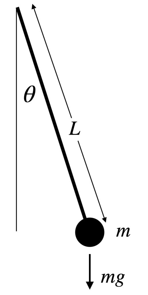
Load ODE
Consider the ODE:
Define the class for the ODE to be integrated. In this case the class
PendulumODE derived from the base class ODEsystem. The following code is
the contents of the file PendulumODE.m cleared of comments and unnecessary
lines:
% Class container for the pendulum
classdef PendulumODE < ODEsystem
  %
  properties (SetAccess = protected, Hidden = true)
    m_m;   % Pendulum mass (kg)
    m_l;   % Pendulum length (m)
    m_g;   % Gravity acceleration (m/s^2)
    m_X_0; % Initial conditions
  end
  %
  methods
    %
    % - - - - - - - - - - - - - - - - - - - - - - - - - - - - - - - - - - -
    %
    function this = PendulumODE( m, l, g, X_0 )

      CMD = 'PendulumODE::PendulumODE(...): ';

      % Set the number of equations and the number of invariants
      num_eqns = 2;
      num_invs = 1;

      % Call the superclass constructor
      this@ODEsystem('PendulumODE', num_eqns, num_invs);

      % Check the input arguments
      assert(m > 0, ...
        [CMD, 'pendulum mass must be positive.']);
      assert(l > 0, ...
        [CMD, 'pendulum length must be positive.']);
      assert(g > 0, ...
        [CMD, 'gravity acceleration must be positive.']);
      assert(length(X_0) == 2, ...
        [CMD, 'initial conditions must be a 2-vector.']);

      this.m_m   = m;
      this.m_l   = l;
      this.m_g   = g;
      this.m_X_0 = X_0;
    end
    %
    % - - - - - - - - - - - - - - - - - - - - - - - - - - - - - - - - - - -
    %
    function out = F( this, x, x_dot, ~ )

      CMD = 'PendulumODE::F(...): ';

      % Check the input arguments
      assert(length(x) == this.m_num_eqns, ...
        [CMD, 'invalid x vector length.']);
      assert(length(x_dot) == this.m_num_eqns, ...
        [CMD, 'invalid x_dot vector length.']);

      % Evaluate the system
      out    = zeros(2,1);
      out(1) = x_dot(1) - x(2);
      out(2) = x_dot(2) + this.m_g / this.m_l * x(1);
    end
    %
    % - - - - - - - - - - - - - - - - - - - - - - - - - - - - - - - - - - -
    %
    function [JF_x, JF_x_dot] = JF( this, ~, ~, ~ )

      % Evaluate the system Jacobians
      JF_x      = zeros(2);
      JF_x_dot  = eye(2);
      JF_x(1,2) = -1.0;
      JF_x(2,1) = this.m_g / this.m_l;
    end
    %
    % - - - - - - - - - - - - - - - - - - - - - - - - - - - - - - - - - - -
    %
    function out = H( this, x, ~ )
      out = [];
    end
    %
    % - - - - - - - - - - - - - - - - - - - - - - - - - - - - - - - - - - -
    %
    function out = JH( this, x, ~ )
      out = [];
    end
    %
    % - - - - - - - - - - - - - - - - - - - - - - - - - - - - - - - - - - -
    %
  end
  %
end
Instantiate the ODE
Having PendulumODE.m now can instantiate a ODEsystem class instance with
the desired parameters, e.g. mass, length, gravity and initial conditions:
% Pendulum parameters
m = 1.0;  % mass (kg)
l = 1.0;  % length (m)
g = 9.81; % gravity (m/s^2)

% Initial conditions
theta_0 = 5*pi/180;
omega_0 = 0.0;
X_0     = [theta_0, omega_0];

ODE = PendulumODE(m, l, g, X_0);
Choose solver
Choose ExplicitEuler and RadauIA5 as solvers and attach the
instantiated ODEsystem to them:
solver1 = ExplicitEuler();
solver2 = RadauIA5();
solver1.set_ode(ODE);
solver2.set_ode(ODE);
Integrate
Select the range and the desired sampling steps for the numerical solution:
d_t   = 0.05; % Desired time step (s)
t_ini = 0.0;  % Initial time (s)
t_end = 10.0; % Final time (s)
T_vec = t_ini:d_t:t_end;
Compute numerical solution using the solve method of the solvers:
[X1, T1] = solver1.solve(T_vec, X_0);
[X2, T2] = solver2.solve(T_vec, X_0);
Now the matrices X contain the solution of the system of ODEs at each time
step in the vectors T. The vectors X are matrices where the first row
contains \(\theta\), and the second row contains \(\omega\) values at
each time step. Notice that the vectors T are not necessarily the same as
T_vec since the solvers may choose to sample the solution at different time
steps.
Extract solution
To extract the solution at each time step, use the following code:
time  = T1;
theta = X1(1,:);
omega = X1(2,:);
x     =  l*sin(theta);
y     = -l*cos(theta);
this will give you the solution at each time step in the vectors time,
theta, omega, and the cartesian coordinates of the pendulum in the
vectors x, and y.
Plot the solution
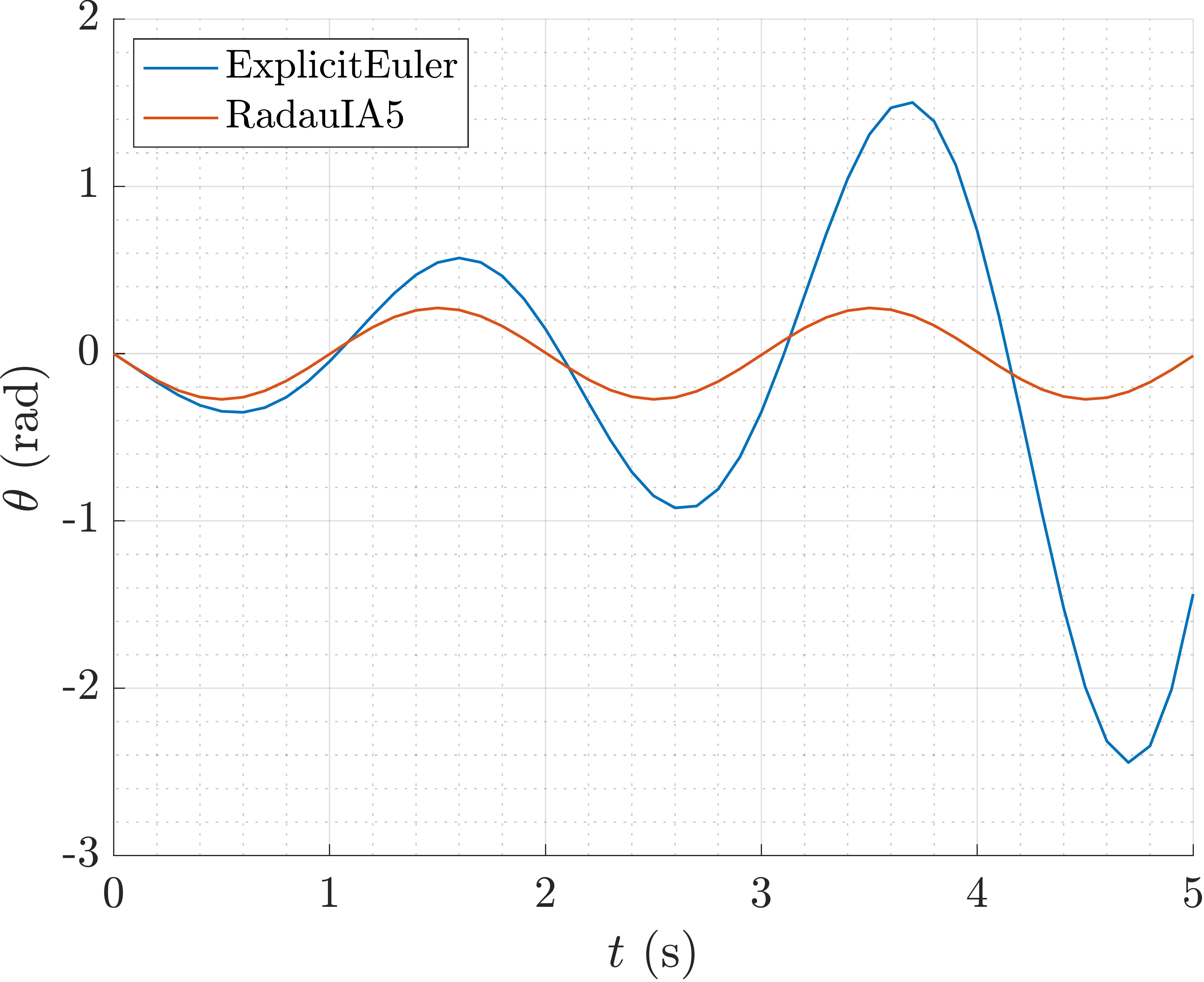
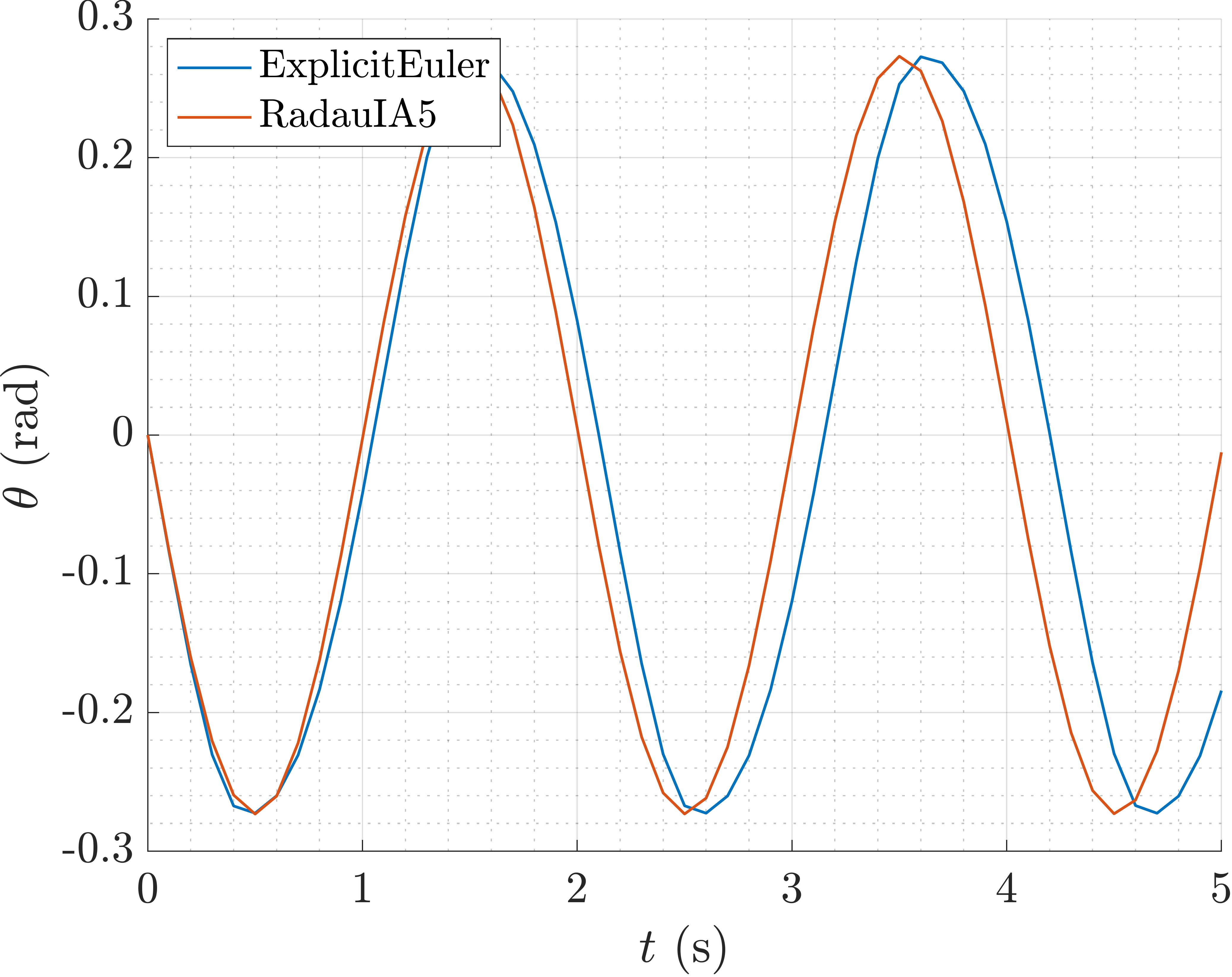
Plot of the angle \(\theta(t)\) .
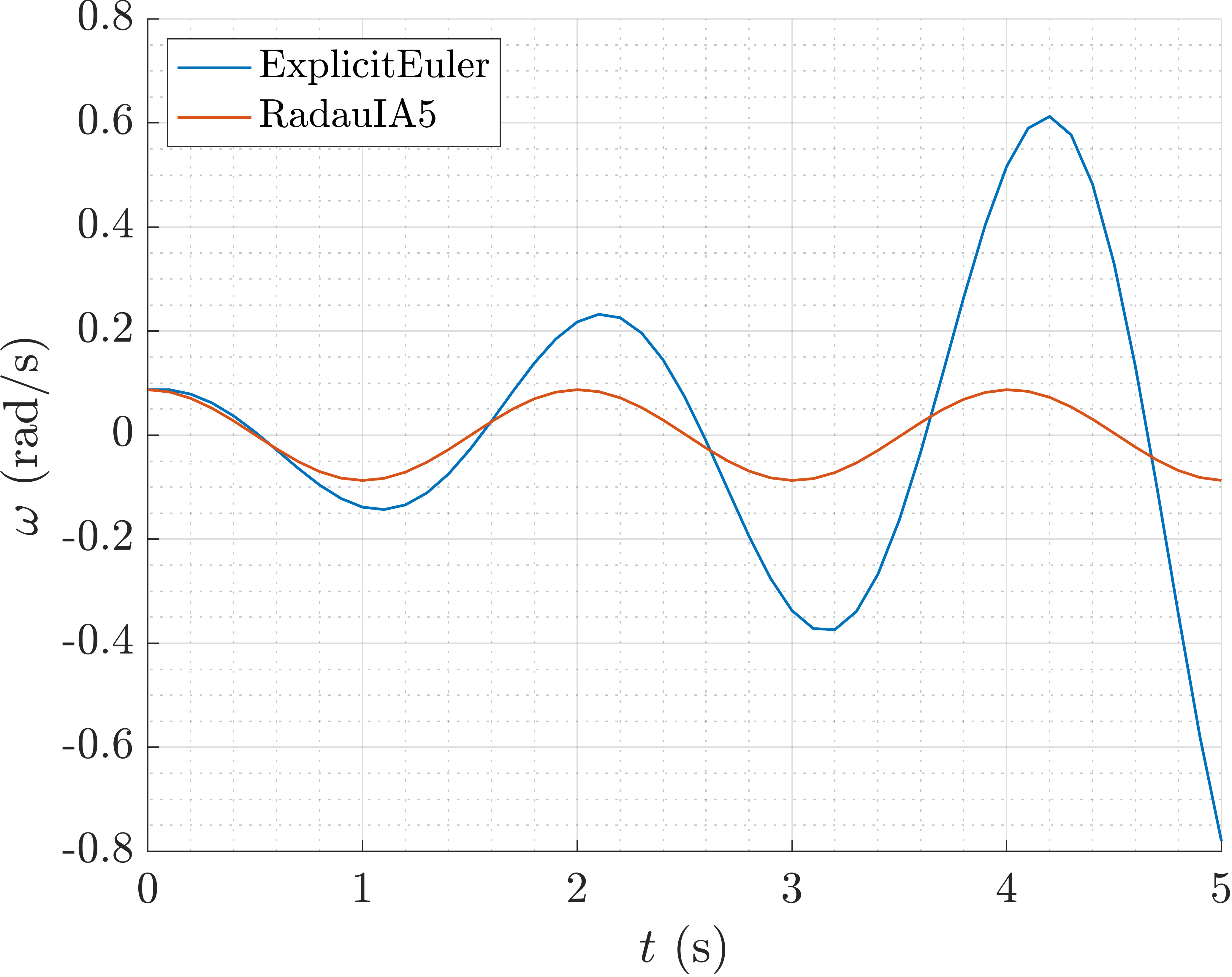
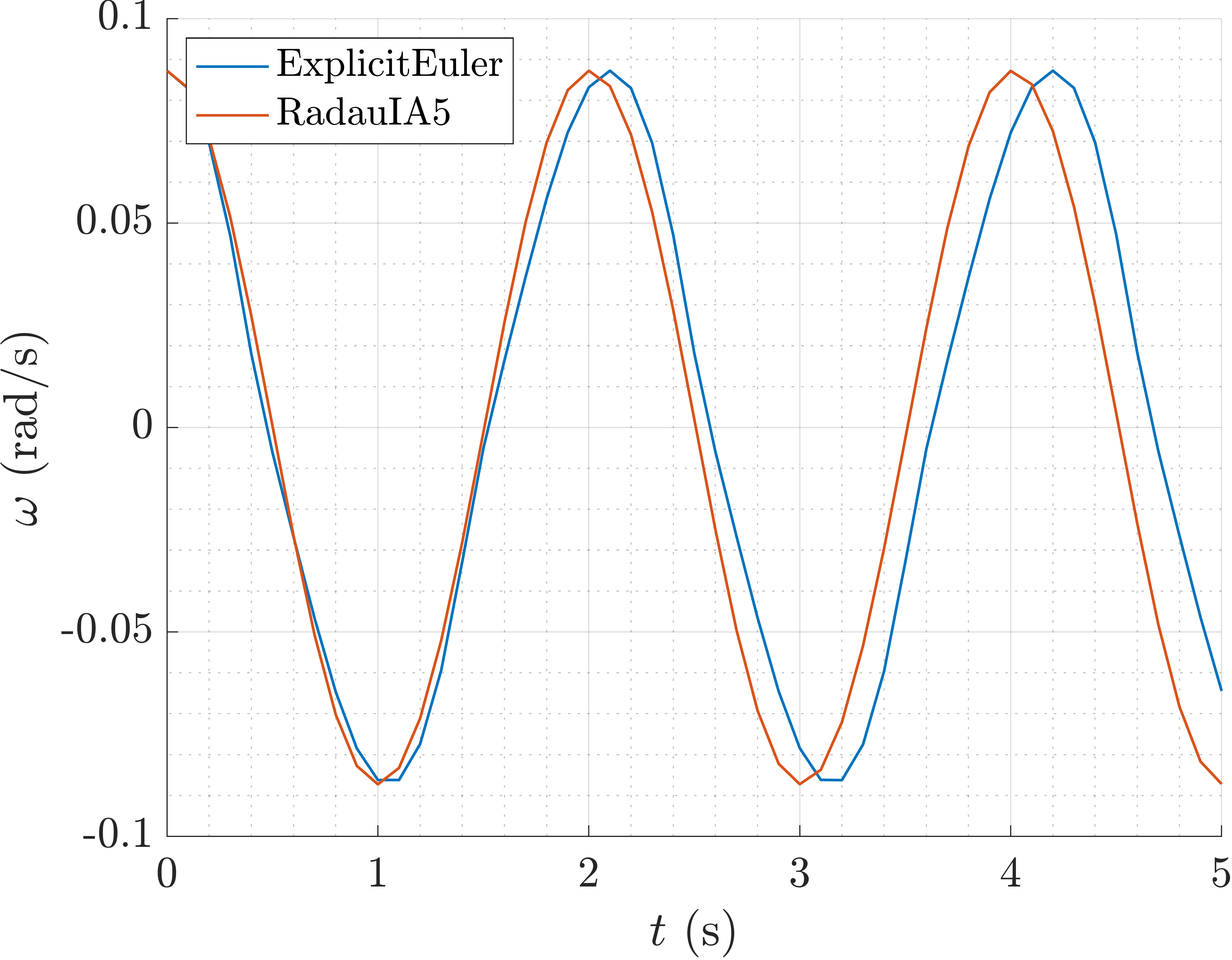
Plot of the angular velocity \(\omega(t)\) .
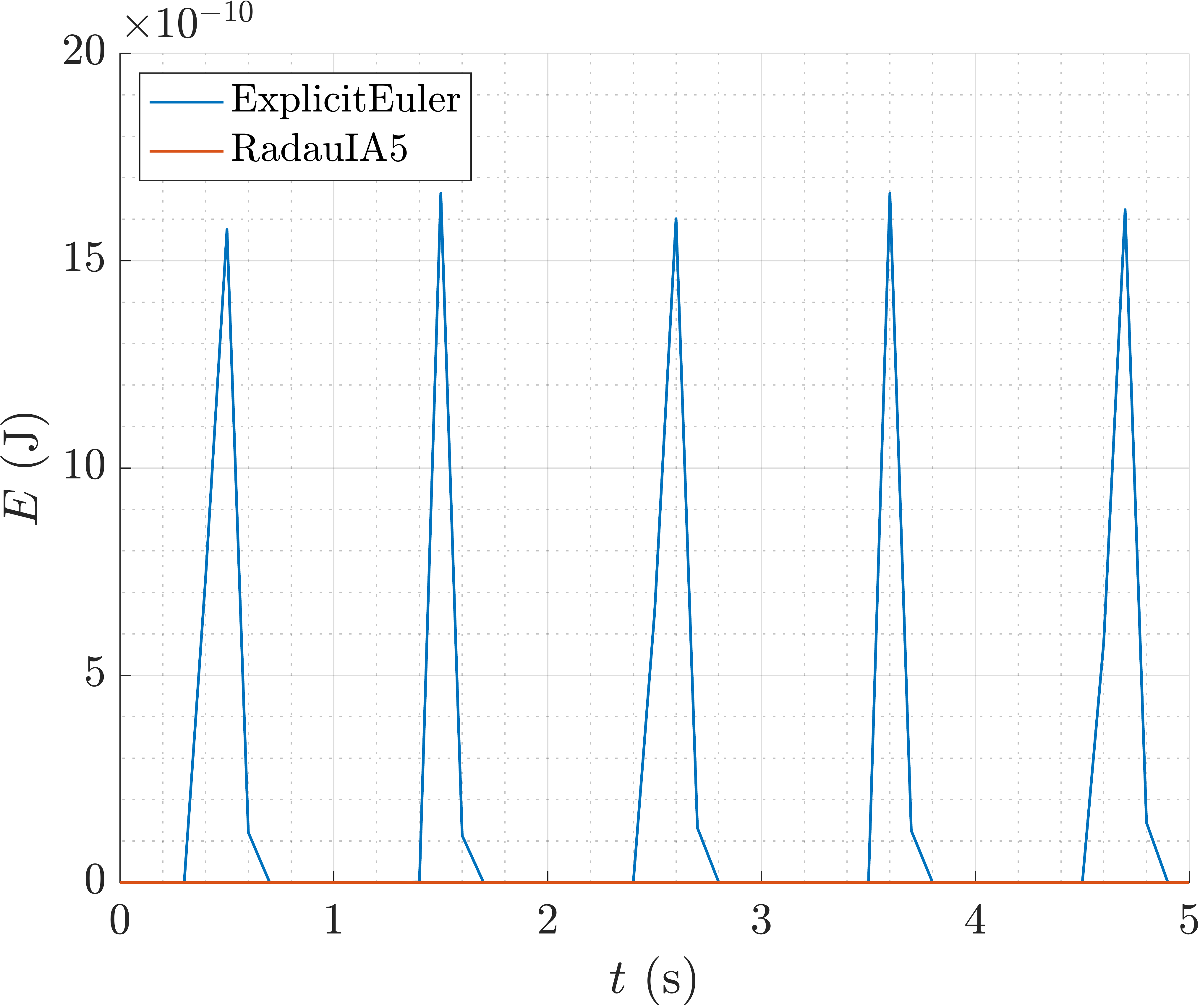
Plot of the energy \(E(t)\) .
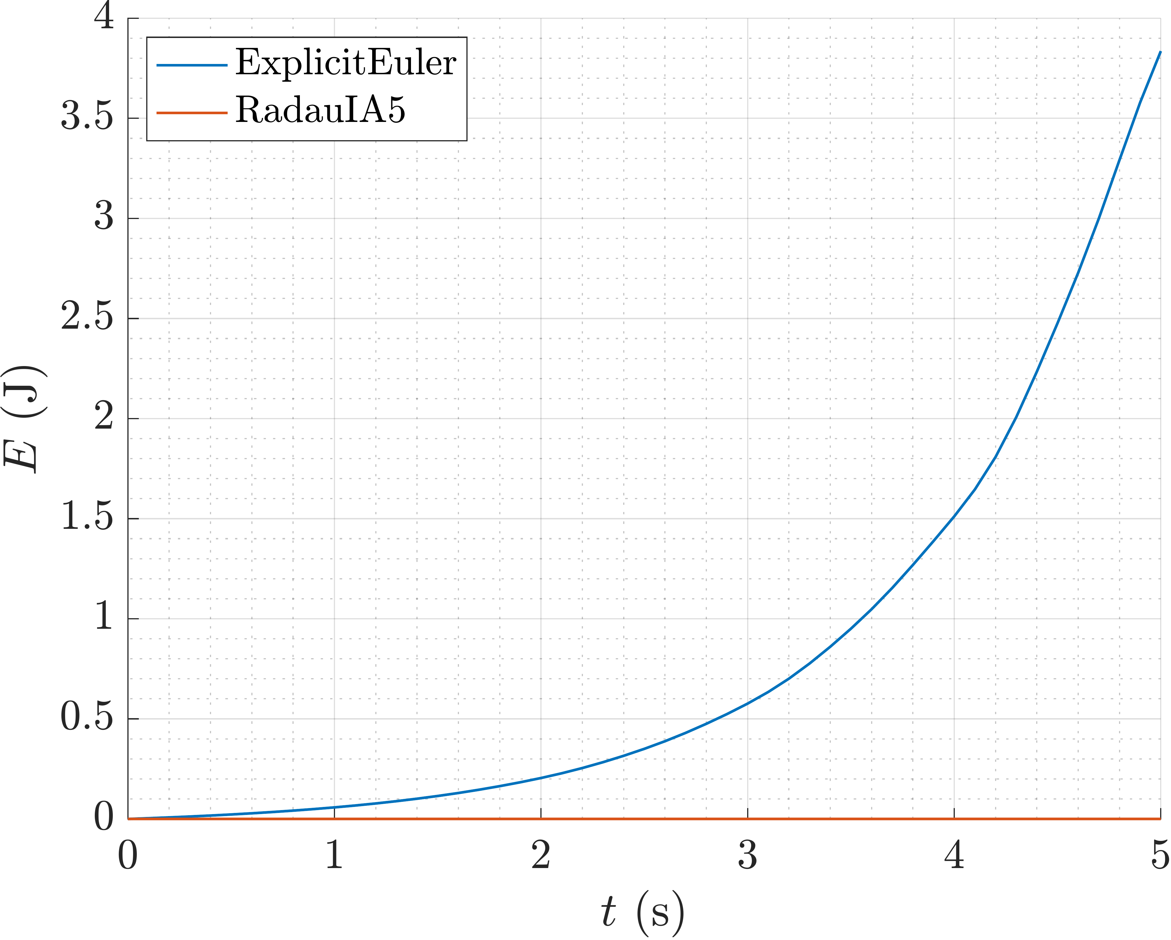
As we can notice the solution is drifting away from the exact solution. This is
due to the fact that when solving the system of ODEs we are using a numerical
method, and the numerical method is not exact. The numerical method is only
approximating the solution of the system of ODEs. The numerical error can be
controlled by choosing a smaller time step d_t or by using a more accurate
numerical method. In addition to that, the numerical error can be reduced by
enhancing the class PendulumODE with the invariants of the system of
ODEs, e.g. the energy of the system, which can be used to correct the numerical
solution at each time step.
Invariants and Projection
Invariants are quantities that are conserved in the system of ODEs. In the case of the linear pendulum, the energy of the system is conserved. The energy (or invariant) of the system is given by:
Its derivative with respect to the states of the system is the invariant of the system:
The energy of the system is a function of the state of the system, i.e. the
angle \(\theta\) and the angular velocity \(\omega\). In order to use
the variation of energy of the system as an invariant, we need to define the
method H in the class PendulumODE to compute the invariant of the system
at each time step:
function out = H( this, x, ~ )

  CMD = 'PendulumODE::H(...): ';

  % Check the input arguments
  assert(size(x,1) == this.m_num_eqns, ...
    [CMD, 'invalid x vector length.']);

  % Evaluate the system invariant
  out = this.m_m.*this.m_g.*this.m_l.*(cos(this.m_X_0(1))-cos(x(1,:))) + ...
        0.5.*this.m_m.*this.m_l^2.*(x(2,:)).^2;
end
and to compute its derivative with respect to the states of the system to obtain
the method JH:
function out = JH( this, x, ~ )

  CMD = 'PendulumODE::JH(...): ';

  % Check the input arguments
  assert(size(x,1) == this.m_num_eqns, ...
    [CMD, 'invalid x vector length.']);

  % Evaluate the system gradient of the invariant
  out = [this.m_m.*this.m_g.*this.m_l.*sin(x(1,:)), ...
        this.m_m.*this.m_l^2.*x(2,:)];
end
Now we can use the variation of the system energy as an invariant to correct the numerical solution at each time step. To do so, we enable the projection in the solution process:
[X, T] = solver.solve(T_vec, X_0, true);
The plots of the angle and the angular velocity are now much better even with a
simple numerical method like ExplicitEuler:
Plot of the projected angle \(\theta(t)\) .
Plot of the projected angular velocity \(\omega(t)\) .
Plot of the projected energy \(E(t)\) .
Note that also the natural frequency of the system is not matched by the
numerical solution of the ExplicitEuler method. To incresase the accuracy
of the numerical solution, we can use either a more accurate numerical method like
RungeKutta4 or a smaller time step d_t.
